Task Definition

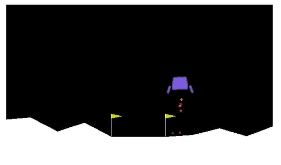
The task accomplished by this project is to build an AI agent for the game of Lunar Lander defined by openAI gym in Box2D format. Here, a lunar lander needs to land with zero velocity between the flags on a landing pad as shown in the figure. with a constant high reward. This is accomplished by Reinforcement Learning, particularly by applying different Deep Q-learning techniques. This project has explored DQN[@journals/nature/MnihKSRVBGRFOPB15], Double DQN[@DoubleQ-learning], and Dueling DQN[@Dueling], to solve the game. We consider the game as solved when the agent starts getting an average reward of 200 over 100 consecutive episodes. Moreover, the performance of different DQN variants are compared to solve the problem.\

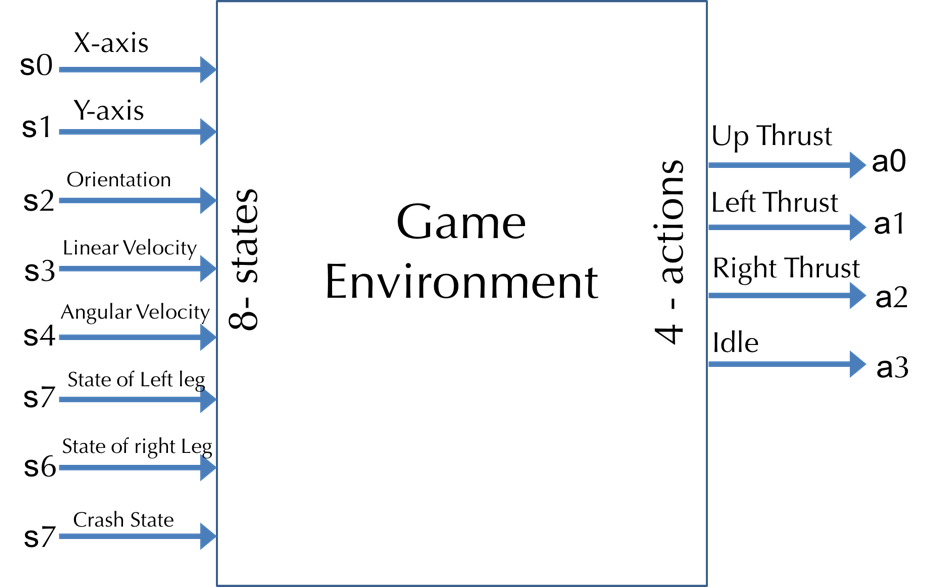
Since, the problem involves high dimensional and continuous state space, standard Q-learning cannot solve this problem unless some amount of discretization is done. Due to this difficulty, Deep Q-Network (DQN) was the choice.

Infrastructure

We have used the OpenAI gym [@openai] library to train our agent. Although some insights are provided in Box2D Lunar Lander on the OpenAI website, thorough exploration of actions, state space, environment etc. was done before starting to solve the problem. Following is the description:

Actions

In this game, four discrete actions are available to the playing agent at any time frame:

1. Do nothing

2. Fire left orientation engine (rotates the lunar lander clockwise)

3. Fire main engine (provides upward thrust)

4. Fire right orientation engine (rotates the lunar lander anti-clockwise)

The agent can choose only one action among the given actions at a given time frame.

Terrain

The terrain is a combination of 10 points, and the helipad(landing zone) is fixed between 5th and 6th points towards the center. The values of the height of the landing zone(5th and 6th points on the terrain) are viewport height divided by 4, and the rest of the points are randomly sampled between 0 to H/2 using numpy random and smoothened (averaging 3 continuous points).

State

The state is 8 dimensional values of different parameters of the lunar lander at any given time. The starting state is randomly initialized (the lunar lander takes a step in the world through the "idle" action) with certain bounds based on the environment. The state space is as follows

1. Position of LunarLander w.r.t X-axis

2. Position of LunarLander w.r.t Y-axis

3. Velocity along X-axis

4. Velocity along Y-axis

5. LunarLander Angle

6. Angular velocity

7. Left leg contacted the surface (Initial value: False)

8. Right leg contacted the surface (Initial value: False)

End State

When the lunar lander stabilises on the landing surface (change in shape of lunar lander is constantly 0 for a number of frames and speed is 0).

Rewards and Transitions

Before defining the rewards, let's define the shape of the lunar lander which decides the rewards. The shape of the lunar lander is a function of position coordinates $(x, y)$, linear velocities $(v_x, v_y)$, lander angle $\theta$ and contact of both the lander legs. We are interested in finding the change of shape at every step for the lunar lander to calculate the rewards for each given action. Shape change is given by subtraction of previous shape and current shape. Formally, shaping at time frame $t$:

$$\begin{aligned} \text{shaping}_{t} = &- 100*(x^2 + y^2) \\ & - 100*(v_x^2 + v_y^2) \\ &- 100*abs(\theta) + 10*(\text{Left leg contacted}) + 10*(\text{Right leg contacted}) \\ \text{shape change} = & \text{shaping}_t - \text{shaping}_{t-1} \end{aligned}$$

The rewards are defined as follows:

1. If the lunar lander crashes, or goes out of the bounds: $-100$

2. If the lunar lander is not awake anymore (stabilises at 0 shape change): $+100$

3. Doing nothing: shape change

4. Firing the engine: shape change - 0.3

5. Rotating: shape change - 0.03

The total reward will automatically be a sum of all the rewards at each time frame, and if the lander touches the ground with it's legs, will add those rewards to the total rewards earned during an episode. Transition probabilities are unknown, we get next states by simulating the lunar lander in the box environment given the current state and action taken.
Note: The transition probabilities and rewards are unknown to our agent, which it will try to figure out through exploration and incorporate in learning.

Models and different Approaches

Q-Learning and DQN

Q-Learning learns the action-value function Q(s,a) which gives us a measure of how good it is to take an action at a particular state. Function Q(s, a) is defined such that for given state $s$ and action $a$ it returns an estimate of a total reward we would achieve by taking the action. Let's call the Q function for the optimal policies $Q_{opt}$. $Q_{opt}$ with discounting can be written as $Q_{opt}(s,a) = r_{0} + \gamma r_{1} + \gamma^{2} r_{2} + ...$ Here, $r$ stands for rewards. $\gamma$ is called a discount factor and when set it to $\gamma <$ 1 , it makes sure that the sum in the formula is finite. The $\gamma$ controls how much the function Q in state $s$ depends on the future and so it can be thought of as how much ahead the agent sees. The above equation can be rewritten in a recursive form. $Q_{opt}(s,a) = r_{0} + \gamma max_{a}Q_{opt}(s',a)$ This equation is proven to converge to the desired $Q_{opt}$, with finite number of states and each of the state-action pair is presented repeatedly.

In Q-Learning we build a memory table Q[s,a] to store Q-values for all the possible combinations of s and a. However, for Lunar Lander the combinations of state and actions are too large and continuos, the memory requirements for Q will be too high. To address this we switch to a deep Q network to approxiamate Q(s,a) using deep neural network. Model-free based Deep Q-learning Network algorithm was chosen specifically for the state size and complexity to approxiamate state-action value function, Q(s, a).

Challenges in RL

As compared to Supervised learning where samples are independent and identically distributed (i.i.d) using randomization among batches. This kind of stable condition for input and ouput ensures supervised model to perform well. In Reinforcement Learning , both the input and output are changing constantly during the training process and makes training unstable. Also, there is another problem related to the correlations i.e. while training we update model parameters to move Q(s,a) closer to ground truth (best action). These parameter update will impact other estimations and cause overfitting.

Implementation Details for DQN

Experience Replay

We put the last state transitions into a buffer memory and sample a mini-batch of samples(batch size) from this buffer to train the deep network. This forms an input dataset which is stable enough for training. As we randomly sample from the replay buffer, the data is more independent of each other and closer to i.i.d. The key idea of 'experience replay' is that we store these $(s, a, r, s')$ transitions in a memory and during each learning step, sample a random batch and perform a gradient descend on it. After reaching the finite allotted memory capacity, the oldest sample is discarded.

Target Network

We create two deep networks. We use the first one to retrieve Q values while the second one includes all updates in the training. This network is a mere copy of the previous network, but frozen in time. It provides stable $\tilde{Q}$ values and allows the algorithm to converge to the specified target: $Q(s, a) \xrightarrow{} r + \gamma max_a \tilde{Q}(s', a)$

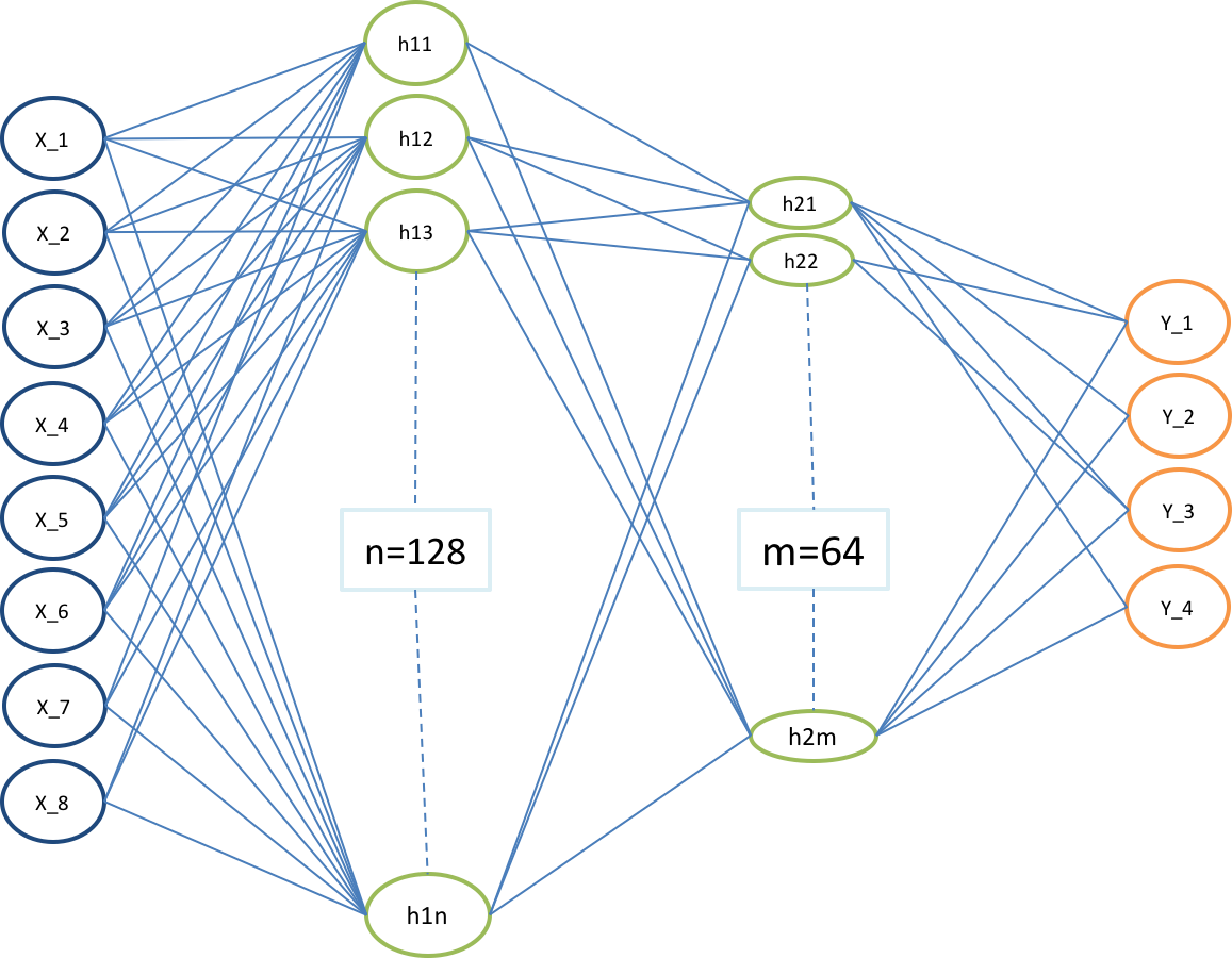
After several steps, the target network is updated, just by copying the weights from the current network. To be effective, the interval between updates has to be large enough to leave enough time for the original network to converge. For lunar lander, we update target model after every episode. We used the Neural Network shown in Fig 2 for Lunar Lander.

Exploration

To find out that actions which might be better then others, we use $\epsilon$ greedy policy. This policy behaves greedily most of the time, but chooses a random action with probability $\epsilon$.

Improvements to DQN

To overcome this problem, researches proposed to use a separate target network for setting the targets. From here on whenever we refer to DQN we mean Full DQN.

Double DQN

One problem in the DQN algorithm is that the agent tends to overestimate the Q function value, due to the max in the formula used to set targets. Because of the max in the formula, the action with the highest positive/negative error could be selected and this value might subsequently propagate further to other states. This leads to bias -- value overestimation. This severe impact on stability of the learning algorithm. In this new algorithm, two Q functions $Q_{1}$ and $Q_2$ -- are independently learned. One function is then used to determine the maximizing action and second to estimate its value. Either $Q_1$ or $Q_2$ is updated randomly with a formula: $Q_1(s, a) \xrightarrow{} r + \gamma Q_2(s', argmax_a Q_1(s', a))$ or $Q_2(s, a) \xrightarrow{} r + \gamma Q_1(s', argmax_a Q_2(s', a))$ It was proven that by decoupling the maximizing action from its value in this way, one can indeed eliminate the maximization bias. When thinking about implementation into the DQN algorithm, we can leverage the fact that we already have two different networks giving us two different estimates Q and $\tilde{Q}$ (target network). Although not really independent, it allows us to change our algorithm in a really simple way. The original target formula would change to: $Q(s, a) \xrightarrow{} r + \gamma \tilde{Q}(s', argmax_a Q(s', a))$ We could observe that Double DQN was more stable than Full DQN.

Dueling layer DQN

In Dueling DQN, Q is computed with a different formula below with value function V and a state-dependent action advantage function A below:

$Q(s,a) \rightarrow V(s) + A(s,a) -\frac{1}{A} \sum_{a'}^{} A(s,a )$

Instead of learning Q, we used two separate heads to compute V and A.Our experiments show the performance improvements. DQN updates the Q-value function of a state for a specific action only. Dueling DQN updates V which other Q(s, a') updates can take advantage of also. So each Dueling DQN training iteration is thought to have a larger impact.
The insight behind the dueling network architecture is that sometimes the exact choice of action does not matter so much, and so the state could be more explicitly modeled, independent of the action. There are two neural networks --- one learns to provide an estimate of the value at every timestep, and the other calculates potential advantages of each action, and the two are combined for a single action-advantage Q function. We can achieve more robust estimates of state value by decoupling it from the necessity of being attached to specific actions.[@Dueling] $Q(s,a) \rightarrow A(s,a) + V(s)$

Accuracy and Efficiency Trade-off

For our solutions, accuracy can be considered as consistency in getting more than 200 scores over a period of episodes. And efficiency would be how sooner we can get such weights for which the agent scores more than 200 scores.
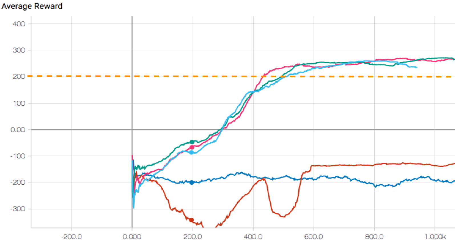
When we train for more number of episodes (low efficiency) we converge better and rewards are consistently better (more than 200), contributing to high accuracy(drop between consecutive episodes is lesser). But if we stop early(at 400 episodes) , we are highly efficient( but the accuracy is lower). It is evident from the smoothness in average rewards post 600 episodes (Tensorboard curve shown in Figure 6).

Experiments and Evaluation

In this section, we will present experimental results for all three different models presented in previous section as well as the visualization of training process.

Baselines

The first baseline is purely a random approach. The Agent was taking random actions and this is just to make sure our agent outperforms a random one. The second baseline is a simple linear classifier.

Oracle

We defined our oracle to be human playing score and the leaderboard scores. In order to create a simulation where humans could actually play the game and collect data, we used openai gym's implementation code. We recorded observations for the same after playing the game 10 times each.
Player 1 2 3 4 5 6 7 8 9 10 Avg. Score

---

Prabhjot $180$ $200$ $-10$ $150$ $20$ $10$ $120$ $130$ $-90$ $-80$ $63$ Abhishek $80$ $100$ $-90$ $-90$ $180$ $120$ $60$ $200$ $210$ $-80$ $69$ Amey $-90$ $170$ $180$ $160$ $30$ $20$ $150$ $-100$ $90$ $30$ $82$

: Human Oracle Scores

We also compared our results with the ones on OpenAI Gym Leaderboard Wiki. In general, the human oracle scores are less because speed of the LunarLander doesn't affect AI agent however it makes the game hard to play for humans.

Literature Review

Since the game of Lunar Lander is available on openAI gym platform, we came across various implementations of it online. We also found a wiki-driven leaderboard [@leaderboard] is available for a small amount of comparative benchmarks. We found Allan Reyes [@allanreyes] work to be well documented. Here the AI agent was trained using simple DQN. We started with the same approach of simple DQN, and after experimenting with hyperparameters we could achieve better results of getting reward of 200 within 525 episodes. Later two more algorithms Double DQN and Duel DQN further enhanced the results. So far, we stand 2nd place on the leaderboard.

Training

In the most proposed models an initial learning rate of $10^{-4}$ was used to initialize training. Adam Optimizer is used for full duration of number of episodes. All models can be trained within 30-40 mins on CPU as input to the neural network is a state vector. All the models were trained for 800 episodes with batch size of 32 or 64. The number of episodes was choosen based on covergence of the loss, while batch size was choosen to be relatively small to get the benefits of stochasticity. We tried different epsilon decay rates to get the best results (Set 4 in Table 2) .

Hyperparameter Tuning

-We tested with different learning rate of 0.01, 0.002, 0.005 and 0.001. We noticed our model gave best result with 0.001
-We also tried different epsilon decay and got the best results at 0.995
-We tried various combinations of batchsize(32, 64 and 128). Of all combinations, we saw best score with batch size of 64 across all models.
An agent with too high of a discount was unable to credit actions to success, far enough in the future. Simply put, it was too myopic. As a result, agents learned how to hover, but never learned how to land. We also observed effect of having smaller replay-memory size. Sometimes a drop in the rewards after model learns is because after many consecutive successes, the replay buffer won't have many failure cases to train on. So, it used to 'forget' how to recover from many failure cases.\

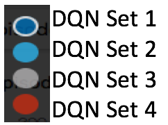
Hyper-parameter Set 1 Set 2 Set 3 Set 4

---

gamma $0.99$ $0.99$ $0.99$ $0.99$
Epsilon(max,min,decay) ($1$,$0$,$.998$) ($1$,$.01$,$.995$) ($1$,$.01$,$.998$) ($1$,$.01$,$.998$)
Learning Rate $0.001$ $0.0001$ $0.0001$ $0.0001$
DNN layers [$32$,$32$] [$128$,$32$] [$128$,$64$] [$128$,$64$]
Loss Function MSE MSE MSE MSE
Batch Size $32$ $32$ $64$ $64$
Replay Memory Size $2^{16}$ $2^{16}$ $2^{16}$ $2^{16}$

: Different set of hyper-parameters were tried

Error Analysis

After doing hyper-parameter tuning, our Agent was able to achieve average score of more than 200 quickly (at 435 episodes). However for some episodes after 435 the rewards were not consistently more than 200 for 100 iterations. This is due to the speed which is not getting reduced to zero (end state) although Lander is in landing zone. The lunar lander is trying to bring itself to a zero velocity state and it tries to do so by applying thrust in opposite direction of landing horizontal velocity. In process of doing this, it applies alternate thrust from left and right side but is not able to bring the lander to complete halt to end the episode. 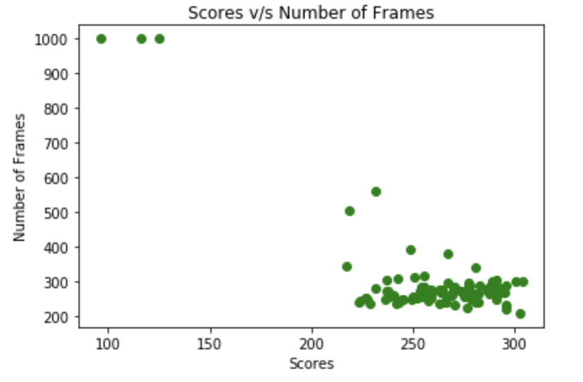Thus reducing the overall rewards and increases the number of frames. We observed that rewards are less than 200 when number of frames reaches the maximum value(1000). The Lunar Lander needs to learn how not to apply alternate left and right thrust to bring itself to a halt, taking no action will be the best action in this state.
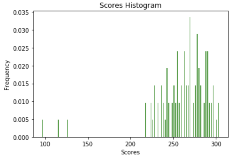
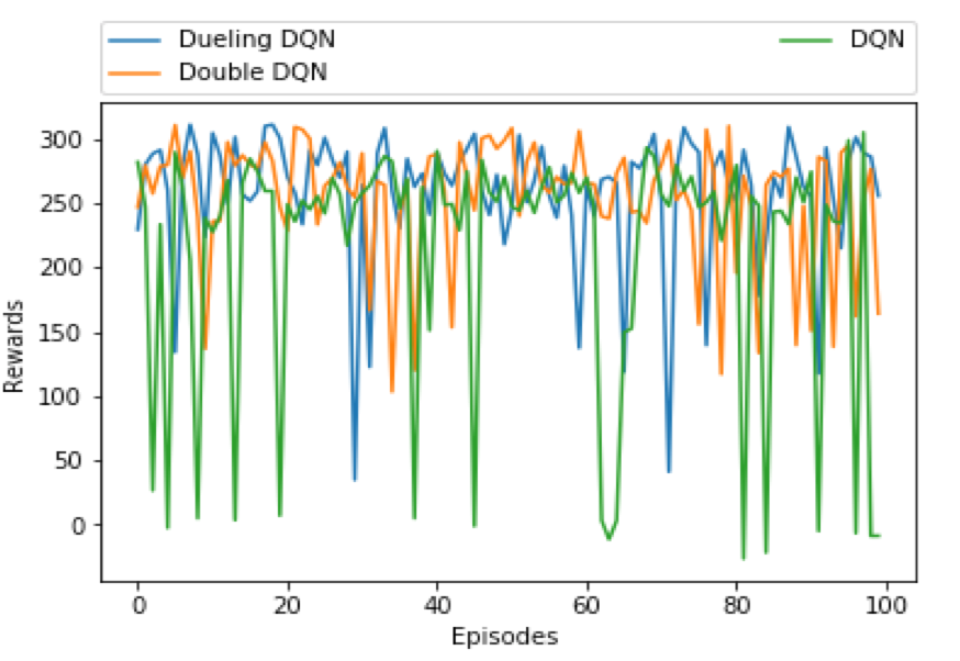
Also, we observe the variation is more in DQN and Double DQN as compared to Dueling DQN. We got the best performance on Set 4 with Dueling DQN model.From figure 5, we can see that the agent underperforms about 4 % of the time. Basically for these 4 cases, the game terminates because we have reached max frame count value (1000). This loss can be attributed to some unexplored states,

Comparision of DQN Variants

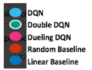
Figure 6 shows comparison of different learning algorithms. The learning performance of baselines are also depicted in the same figure. From the figure, we can see that Dueling Network Architecture reaches the average reward 200 earlier than DQN and Double DQN, near episode number 450. After reaching the reward 200, the graph is getting closer to zero slope. This is also intuitive since after reward 200, the average reward doesn't change much.
Another thing evident from this is that the average reward for the random baseline fixes to a negative value after 600 episodes and there's no much variation on average reward (although the reward for each episode varies significantly).

Model Avg. Score Number of episodes to reach 200 score

---

Baseline $-200$ never Linear Baseline $-150$ never DQN $123$ $525$ Double DQN $220$ $500$ Dueling DQN $225$ $435$

Model Evaluation

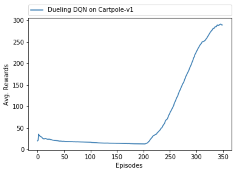
All aforementioned models are evaluated for 100 episodes for a fixed weights as shown in Figure 7(left side).\

Agent on other Environments

We used the Agent to train on "CartPole-v1" game environment and were able to achieve good results. After Our AI agent successfully learnt the game as shown in Figure 7(right side) and consecutively won it. This proves the generality of the algorithm.

Conclusion

We were successful in implementing an AI agent which was able to score an average reward of more than 200 for 100 consecutive episodes and compared different variants of DQN. DQN was applied effectively on this specific problem, and produced successful results.
The DQN variants we tried gave very good results once the hyperparameters were tuned correctly. When implemented the algorithm code in a modularized format, we could easily change the parameters and play with it. Also, minimal tweaks were required for each the DQN variant. Not much of hyperparameter tuning was required across DQN variants. The more advanced Duel Q-learning learner undoubtedly increased the accuracy of the reinforcement learning agent. Given more time and resources, the agent could have been tuned via a more exhaustive grid search. After some literature review, we tried out DQN with Prioritized replay as well. Unfortunately, the results were not promising in comparison to rest of the three approaches.

Codalab Link

https://worksheets.codalab.org/worksheets/0x1e3fc24cfa0d4ff3b492d0f47b6e0887/\ Command to run :\

cl run :brain.py :hyperparameters.py :main.py :agent.py :environment.py :memory.py \

:weights_0450.hdf5 'python3 main.py --should_learn=False --agent=Dueling \

--initial_weights=weights_0450.hdf5' -n Dueling-Log --request-docker-image prabhjotrai/openai-gym:v1

Appendix

Implementation choices

The choice of state was based on the actual configuration of the lunar lander, and we learnt weights for each feature in the state. Another choice could have been training on image data, feeding images per episode and learning on gained rewards. Since this would have been computationally expensive, we chose the former approach to explicit definition of state space and learning it's weights.
For running different algorithms, we created separate classes so that the code is not only modularized, but can also be run easily on different openai environments, learning algorithms can be easily changed etc. Here's a quick description of different classes:

1. Brain: Class which contains keras models, updates the weights through train function and performs prediction based on learnt weights.

2. Memory: Class which appends observations until maximum memory length and samples based on given batch size hyperparameter

3. Agent: Our agent class which explores and exploits based on fixed hyperparameters(gamma, epsilon max, epsilon min and decay) and passed arguments. This is also the class where we are performing the replay action and training the agent's brain instance. It also contains another instance of memory class which is used in replay while sampling.

4. Environment: Class which runs the episode on given agent and asks the agent to observe and replay whenever the agent is trying to learn on episodes. It returns the information on how much reward was observed on each episode and for how long each episode ran