Funded by

Introduction

Due to the advancement of various techniques in machine learning and artificial intelligence, we have seen a corresponding increase in applications of them in different fields. One such application is providing assistance in driving, complementing the drivers and aiding them in various scenarios. Extended applications include partial or fully self driving cars. Most of these Advanced Driver Assistance Systems (ADAS) aim at taking the passengers from location A to location B, following traffic rules and keeping safety of the environment at utmost priority. In this project, we extend such agents by adding time constraints (along with partially relaxing traffic rules constraints such as speed) so that ADAS can be catered towards Emergency Services.

In this project, we trained an agent in an environment simulated in CARLA[2] as it is open source and provided the flexibility to create our own track. The data generated by the simulation was used to train deep reinforcement learning models and their performances were compared for speed and quality of solutions. Specifically, we evaluated the time taken by the agent to complete the created track and the behavior of the reward function under the various algorithms.

CARLA

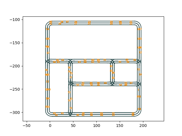
CARLA is an open source simulator specifically designed for autonomous driving research. It is built on top of Unreal Engine, which allows for a realistic graphics simulation of a variety of driving scenarios. CARLA lets the end user control a variety of factors like weather, traffic manager, collision detection, change the kind of maps that the simulation runs on and on how realistic the simulation is. For this course we use CARLA version 0.9.15 and use town a slightly modified version of Town 02 with a lot of scenery removed. Attached below is a birds-eye image of the map with spawn points plotted out for where the different agents can be spawned.

States and Action spaces

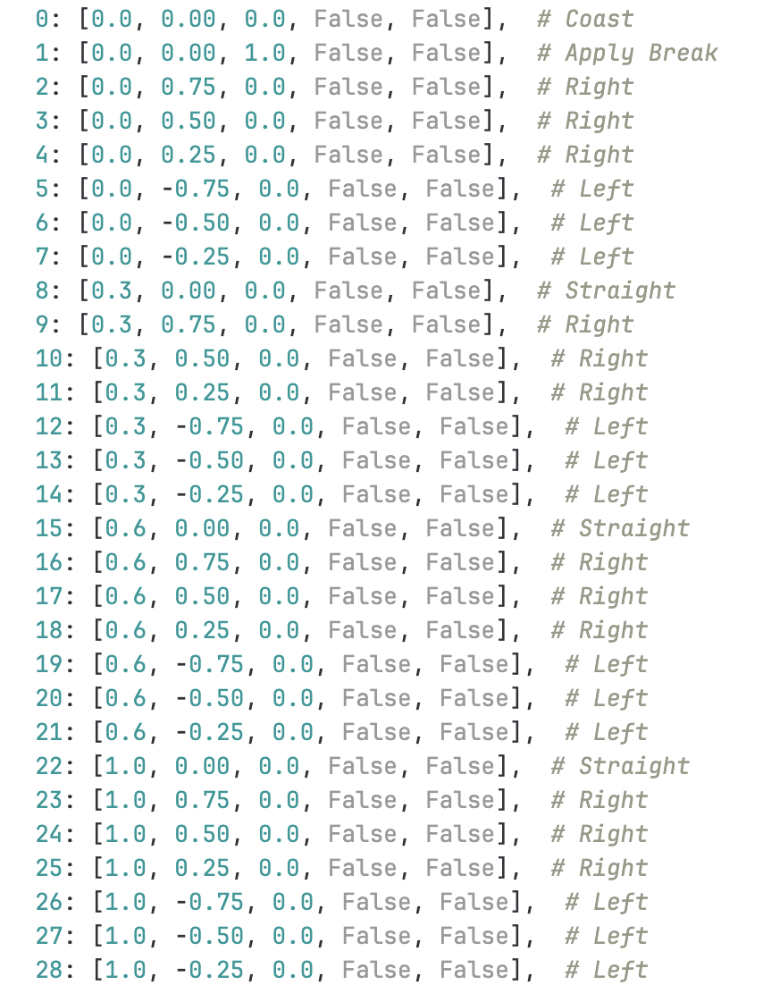
The action spaces used by the agent in CARLA is listed below:

The agent mainly has two states a non terminal and a terminal state - the agent operates the emergency vehicle normally in a non terminal state trying to maximize its rewards while the terminal state of the agent directly correlates to when the agent has crashed with an object at a high intensity resulting in the episode ending early.

Reward function

The reward function for the agent in the CARLA environment has been designed to encourage speed and time, while penalising lane deviation, idle time and fall. The agent has been assigned the following rewards(penalties):

Episodic rewards

• A positive reward proportional to the distance travelled forward
• An additional reward for increase in speed, if the current speed of the vehicle is less than 20, computed as 5% of the speed
• Penalty of 0.5 if the vehicle is not within the given lane
• An additional penalty of 0.4 if there is a significant lateral deviation from the lane and the agent continues to steer in the same direction as the deviation
• A reward of factor (1/time) for reaching the target location sooner

Terminal rewards

• A large penalty of -40 if the vehicle has fallen.
• A large penalty of -100 if the vehicle has been idle for a significant period of time.
• A large negative reward of-100 if the vehicle has reached it’s maximum allowed time.

The substantial penalties, coupled with the episodic rewards, expedite the agent's training process, allowing it to swiftly reach its designated destination by adhering closely to the lane.

Algorithms

Basic Deep-Q Network(DQN)

A DQN is an off-policy reinforcement learning algorithm that learns from past experiences. It employs experience replay, storing past experiences in a replay buffer, allowing for more efficient learning by reusing and learning from these experiences.

A DQN utilizes neural networks to approximate Q-values, where the network learns to estimate the best action to take in a given state. The objective is to minimize the loss function, representing difference between the predicted Q-values and the target Q-values. Using the mean squared error as the loss, the objective function becomes:

$$L(\theta) = \frac{1}{N} \sum_{i=1}^{N} \left(Q(s, a; \theta) - Q_{\text{target}}(s, a)\right)^2$$

The Q-function is parameterized by a neural network with weights. The Q-learning update rule, which is the basis for DQN, is given by

$$Q(s,a)=Q(s,a)+\alpha[r+\gamma max_{a'}Q(s',a';\theta')-Q(s,a)]$$

which represents the target Q-value. The target Q-value is computed using a separate target Q-network, which typically has a different set of parameters from the Q-network being updated. The target network is periodically updated by copying the parameters from the main Q-network. This rule governs how the Q-values are iteratively refined based on new experiences.

The Q-network, with its adjustable parameters, undergoes continuous refinement through backpropagation and optimization, gradually converging towards a more accurate representation of the optimal Q-function.

Soft Actor-Critic

Soft Actor-Critic (SAC) is an off-policy reinforcement learning algorithm characterised by the use of experience replay, that contributes to its off-policy nature. Given the continuous state space and the large range of actions available to the agent in the ADAS system, it appears to be a suitable choice for training. It is an actor-critic method wherein the actor is a policy network that outputs a probability distribution over actions, allowing for stochasticity in action selection and the critic evaluates the value of state-action pairs.

SAC uses the entropy-regularized reinforcement learning technique. The entropy regularization coefficient explicitly controls the explore-exploit tradeoff, with higher corresponding to more exploration, and lower corresponding to more exploitation. SAC concurrently learns a policy and two Q-functions (For deriving the target values and the predicted values, which helps mitigate maximisation bias). The objective function to be minimised is as follows:

$$J(\theta, \phi) = \mathbb{E}_{(s, a, r, s') \sim \mathcal{D}} \left[ \frac{1}{2} \left(Q(s, a; \theta) - (r + \gamma \min_{a'} Q_{\text{target}}(s', a'; \theta^-))\right)^2 \right] - \alpha \ \mathbb{E}_{s \sim \mathcal{D}} \left[ \mathbb{E}_{a \sim \pi_\phi(\cdot|s)}[\text{log}(\pi_\phi(a|s))]\right]$$

Proximal Policy Optimisation

PPO is an on-policy reinforcement learning algorithm that learns directly from the current policy. It implements a form of policy gradient ascent with a trust region constraint, limiting the policy update to prevent large deviations from the current policy.

One of the key innovations of PPO is the use of a clipped surrogate objective. Rather than updating the policy based on the entire advantage function, PPO clips the surrogate objective to prevent large policy updates. This helps to stabilize training and avoid excessively changing the policy.

PPO also often employs an actor-critic architecture, where a policy network (actor) selects actions and a value network (critic) estimates the value of state-action pairs. PPO typically updates parameters to minimise the objective function using mini-batch updates.

PPO introduces an adaptive penalty on the Kullback-Leibler (KL) divergence between the new and old policies. The probability ratio between the new policy and old policy is given by:

$$\rho(\theta) = \frac{\pi_{\theta'}(a|s)}{\pi_{\theta}(a|s)}$$

The objective function to be minimise is given by

$$L(\theta) = \mathbb{E}_{t} \left[ \min \left( \rho_t(\theta) A_t, \text{clip}(\rho_t(\theta), 1 - \epsilon, 1 + \epsilon) A_t \right)\right]$$

Packages and libraries

We formulated our environment conforming to the OpenAI gym’s environment class: https://gymnasium.farama.org/api/env/

Our observation space is a 300x300x3 birds eye view camera image. Our action space comprises discrete values of [throttle, steer, brake, reverse, handbrake] (28 different set of values). Step function applies given action (control) to the world. This should return the reward ****and other details. The reset function resets the given environment. We started by applying this idea to windy gridworld and solved it.

We have primarily used RLlib, which is a high-level library built on top of Ray that provides a comprehensive set of tools for developing and training RL agents. It includes various algorithms, neural network components, and utilities to streamline the RL workflow.

Ray facilitates distributed training of RL agents by providing tools for efficient data parallelism and model parallelism.

OpenAI gym facilitiated retreiving data from the CARLA environment, which we could then feed into the RLlib model.

As mentioned in the docs of CARLA, we used a boilerplate repo (https://github.com/carla-simulator/rllib-integration) to have a skeleton. This was only compatible with version 1 of ray, we upgraded it to version 2 and made changes according to our use case and further added experiments for SAC and PPO. Our final repo: https://gitlab.com/rl-umn/adas-e.

For running the model we setup CARLA on one of the CUDA clusters. Further, we created a cluster using ray.io API to which we submitted jobs. Finally, we ran jobs with the agent using different RL algorithms simultaneously.

Observations

Our results and experiments with the agent trained in the CARLA simulation environment have been populated under:

results - Google Drive

Network and Hyperparameters

We used the default algorithm parameters from the Ray rllib library for the DQN, SAC and PPO algorithms, albeit with a few changes as mentioned in dqn_example/dqn_config.py. The default configuration for SAC resulted in the GPU running out of memory, to resolve which we decreased the training batch size from 256 to 128 (mentioned here: https://docs.ray.io/en/latest/_modules/ray/rllib/algorithms/sac/sac.html#SACConfig). We ran this for rollout worker 1 (which in RLlib context is the agent who performs the episode).

The neural network architecture used is a convolutional neural network, with seven kernels and a feed forward network with two fully connected layers with 256 and 512 neurons. We used a batch size of 64 and replay buffer size of 5000.

Performance of the DQN algorithm

As a preliminary step, we trained a basic DQN model using data generated by simulating the agent in CARLA, using the reward function as described in the “Rewards” section.

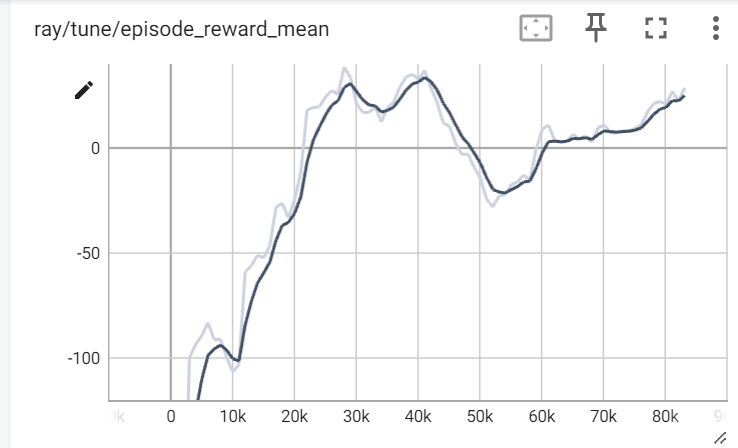
We observe that the mean reward per episode for an agent trained on the DQN converges in about 83,000 iterations, with the maximum episodic reward of 28.62. There is a fairly steep increase in rewards from the 10,000th iteration to the 30,000th iteration indicating a significant learning occurring. There is a small dip around the 52,000th timestep, potentially due to the halting of the agent despite learning to follow a lane.

Rewards per episode

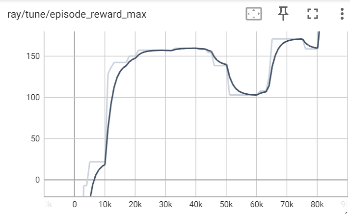
We observe a similar trend in the max reward per episode, with a slightly more sharp increase in the 20,000th timestep.

Performance of the SAC algorithm

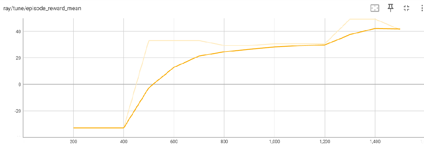
We observe that the SAC algorithm converges in about 1,500 iterations, which is about 1/50 times that of the steps taken by DQN, thereby proving it’s suitability to continuous state spaces and efficacy of the off-policy algorithm. The mean reward per episode was about 41.83, higher than that generated by DQN. The increase in the rewards was gradual from the 400th iteration.

The maximum reward appears to follow a similar trend compared to the mean reward, with the value being 123.63.

Performance of Proximal Policy Optimisation (PPO)

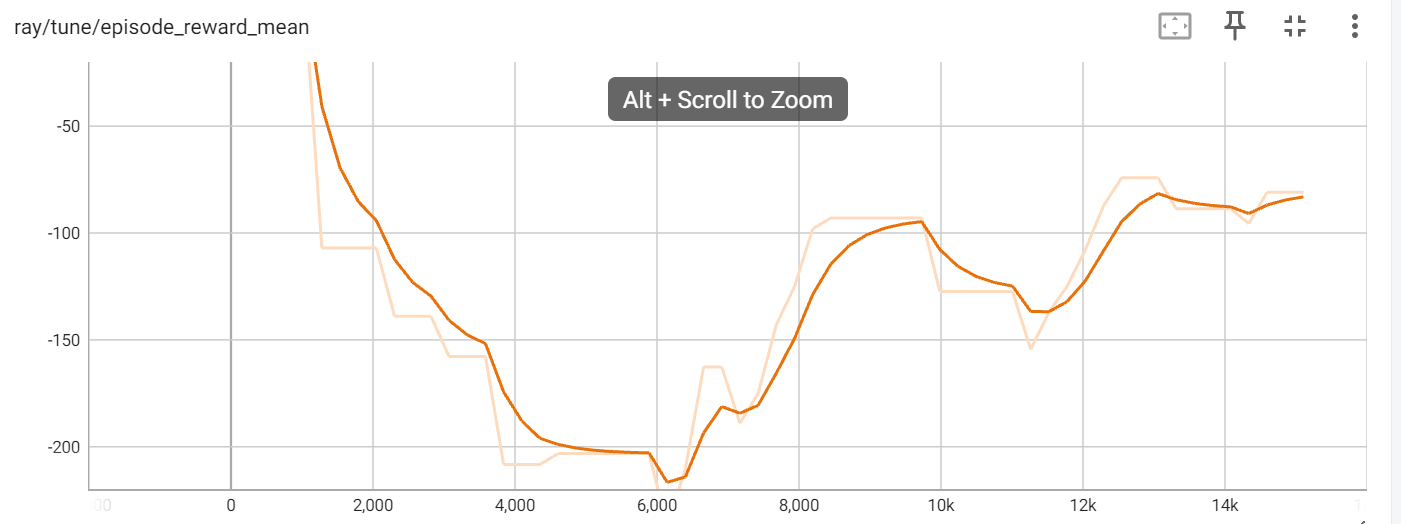
The agent trained by the PPO performed better than DQN as it converged in 14,000 iterations, however SAC appears to be the fastest.

The mean average reward per episode of the PPO trained agent is -81.05.

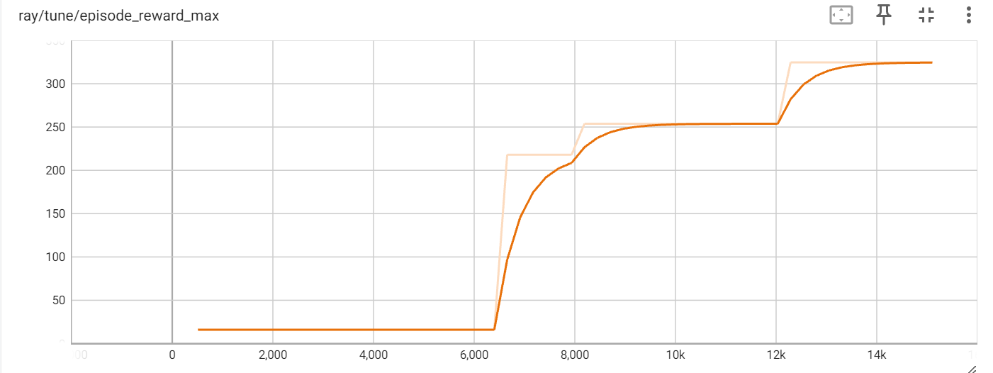
The maximum reward for the PPO agent is consistently increasing, with a value of 324.53.

Behaviour of the agent under optimal policy

Given in the below link is a video tracking the behaviour of the agent under the optimal policy generated by the DQN algorithm.

https://drive.google.com/file/d/1ZMxR43eCU2D7f6Bpj_xvGMqldfRuz5ML/view?usp=drive_link

Based on a visualisation of the behaviour of the agent under the policy with the help of checkpoints, we understand that the agent prioritises speed over lane discipline. This is attributable to the high reward assigned to speed (+100) as compared to the penalty for not sticking to the lane (-0.5). Also, since time is a priority (1/time reward addition), the agent finds out a “shortcut” to the target location instead of following the lane since that’s of top priority.

Finally, the terminal reward did not only involve crossing the finish line but accounted for the speed at the final location. So it would ideally have to slow down near the finish line.

Training the model on AWS DeepRacer

We trained the agent in AWS DeepRacer with model 1 rewards focused on following the centerline, model 2 rewards focused on avoiding zig zag and model 3 rewards targeted to follow the centerline and an extra reward for increasing speed. Model 3 also assigned a higher reward for being closer to progress completion.

However, similar to the limitations faced while training our agent, it appears that the agent was focused on reaching the destination compared to sticking to the lane, on account of which we achieved a US leaderboard score of 222/256.